38 display data labels in excel

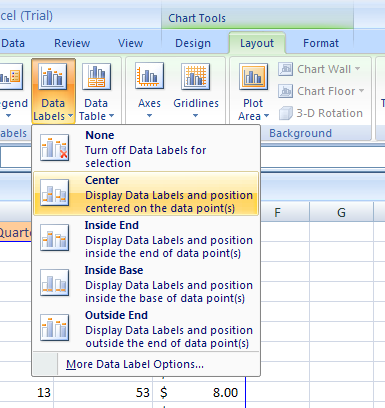
The Art of Dynamic Labeling in Excel - dummies On the Insert tab in the Ribbon, select the Text Box icon. Click inside the chart to create an empty text box. While the text box is selected, go up to the formula bar, type the equal sign (=), and then click the cell that contains the text for your dynamic label. The text box is linked to cell C2. You'll notice that cell C2 holds the Filter ... How to add or move data labels in Excel chart? - ExtendOffice 2. Then click the Chart Elements, and check Data Labels, then you can click the arrow to choose an option about the data labels in the sub menu. See screenshot: In Excel 2010 or 2007. 1. click on the chart to show the Layout tab in the Chart Tools group. See screenshot: 2. Then click Data Labels, and select one type of data labels as you need ...

How to add data labels from different column in an Excel chart? This method will introduce a solution to add all data labels from a different column in an Excel chart at the same time. Please do as follows: 1. Right click the data series in the chart, and select Add Data Labels > Add Data Labels from the context menu to add data labels. 2.

Display data labels in excel

Office: Display Data Labels in a Pie Chart - Tech-Recipes: A Cookbook ... This will typically be done in Excel or PowerPoint, but any of the Office programs that supports charts will allow labels through this method. 1. Launch PowerPoint, and open the document that you want to edit. 2. If you have not inserted a chart yet, go to the Insert tab on the ribbon, and click the Chart option. 3. Find, label and highlight a certain data point in Excel scatter graph Here's how: Click on the highlighted data point to select it. Click the Chart Elements button. Select the Data Labels box and choose where to position the label. By default, Excel shows one numeric value for the label, y value in our case. To display both x and y values, right-click the label, click Format Data Labels…, select the X Value and ... How to show data label in "percentage" instead of - Microsoft Community Select Format Data Labels Select Number in the left column Select Percentage in the popup options In the Format code field set the number of decimal places required and click Add. (Or if the table data in in percentage format then you can select Link to source.) Click OK Regards, OssieMac Report abuse 8 people found this reply helpful ·

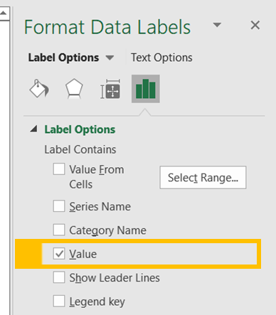
Display data labels in excel. 1/ Select A1:B7 > Inser your Histo. chart. 2/ Right-click i.e. on the 1st histo. bar (A) > Add Data Labels (numbers are displayed a the top of the bars) 3/ Click one of the numbers that just displayed (the Format Data Labels pane opens on the right) > Check option "Value From Cells" > Select range C2:C7 > OK > Uncheck option "Value". Data labels not displayed correctly - Excel Help Forum The data label is a date value that selects values from the date column. The Primary axis is categorized based on 2 values. The secondary axis is Month. The data labels are displayed accurately as per the month except the 3 labels. The first series is the difference between F and E.The second series is the difference between the J and K column. Add or remove data labels in a chart - Microsoft Support Right-click the data series or data label to display more data for, and then click Format Data Labels. Click Label Options and under Label Contains, select the Values From Cells checkbox. When the Data Label Range dialog box appears, go back to the spreadsheet and select the range for which you want the cell values to display as data labels. Quick Tip: Excel 2013 offers flexible data labels | TechRepublic right-click and choose Insert Data Label Field. In the next dialog, select [Cell] Choose Cell. When Excel displays the source dialog, click the cell that contains the MIN () function, and click OK....

5 Ways to Concatenate Data with a Line Break in Excel Sep 15, 2022 · The cell will now display on multiple lines. Conclusions. Excel has many options to combine data into a single cell with each item of data on its own line. Most of the time using a formula based solution will be the quickest and easiest way. We may find ourselves in need of an option which can’t easily be accidentally changed. How to Create Labels in Word from an Excel Spreadsheet In this guide, you'll learn how to create a label spreadsheet in Excel that's compatible with Word, configure your labels, and save or print them. Table of Contents 1. Enter the Data for Your Labels in an Excel Spreadsheet 2. Configure Labels in Word 3. Bring the Excel Data Into the Word Document 4. Add Labels from Excel to a Word Document 5. How to Create Excel UserForm for Data Entry - Contextures Excel … 18-05-2022 · Switch to Excel, and activate the PartLocDB.xls workbook; Double-click on the sheet tab for Sheet2; Type: Parts Data Entry; Press the Enter key; On the Drawing toolbar, click on the Rectangle tool (In Excel 2007 / 2010, use a shape from the Insert tab) In the centre of the worksheet, draw a rectangle, and format as desired. How To Plot X Vs Y Data Points In Excel | Excelchat In this tutorial, we will learn how to plot the X vs. Y plots, add axis labels, data labels, and many other useful tips. Figure 1 – How to plot data points in excel. Excel Plot X vs Y. We will set up a data table in Column A and B and then using the Scatter chart; we will display, modify, and format our X and Y plots.

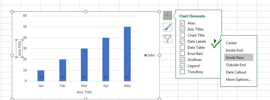
Excel tutorial: How to use data labels Generally, the easiest way to show data labels to use the chart elements menu. When you check the box, you'll see data labels appear in the chart. If you have more than one data series, you can select a series first, then turn on data labels for that series only. You can even select a single bar, and show just one data label. How To Plot X Vs Y Data Points In Excel | Excelchat In this tutorial, we will learn how to plot the X vs. Y plots, add axis labels, data labels, and many other useful tips. Figure 1 – How to plot data points in excel. Excel Plot X vs Y. We will set up a data table in Column A and B and then using the Scatter chart; we will display, modify, and format our X and Y plots. Adding Data Labels to Your Chart (Microsoft Excel) - ExcelTips (ribbon) To add data labels in Excel 2013 or later versions, follow these steps: Activate the chart by clicking on it, if necessary. Make sure the Design tab of the ribbon is displayed. (This will appear when the chart is selected.) Click the Add Chart Element drop-down list. Select the Data Labels tool. How to Create Excel UserForm for Data Entry May 18, 2022 · Switch to Excel, and activate the PartLocDB.xls workbook; Double-click on the sheet tab for Sheet2; Type: Parts Data Entry; Press the Enter key; On the Drawing toolbar, click on the Rectangle tool (In Excel 2007 / 2010, use a shape from the Insert tab) In the centre of the worksheet, draw a rectangle, and format as desired.

Change Chart Data Labels : Chart Data « Chart « Microsoft ...

How to add data labels in excel to graph or chart (Step-by-Step) 1. Select a data series or a graph. After picking the series, click the data point you want to label. 2. Click Add Chart Element Chart Elements button > Data Labels in the upper right corner, close to the chart. 3. Click the arrow and select an option to modify the location. 4.

Excel charts: add title, customize chart axis, legend and ...

Add or remove data labels in a chart - support.microsoft.com Right-click the data series or data label to display more data for, and then click Format Data Labels. Click Label Options and under Label Contains , select the Values From Cells checkbox. When the Data Label Range dialog box appears, go back to the spreadsheet and select the range for which you want the cell values to display as data labels.

Adding rich data labels to charts in Excel 2013 | Microsoft ...

Pandas DataFrame: Create and display a DataFrame from a … 19-08-2022 · Pandas: DataFrame Exercise-2 with Solution. Write a Pandas program to create and display a DataFrame from a specified dictionary data which has the index labels.

Dynamic Number Format for Millions and Thousands - PK: An ...

How to add and customize chart data labels - Get Digital Help Double press with left mouse button on with left mouse button on a data label series to open the settings pane. Go to tab "Label Options" see image to the right. This setting allows you to change the number formatting of the data labels. The image below shows numbers formatted as dates.

Change the format of data labels in a chart

How to Print Labels from Excel - Lifewire Select Mailings > Write & Insert Fields > Update Labels . Once you have the Excel spreadsheet and the Word document set up, you can merge the information and print your labels. Click Finish & Merge in the Finish group on the Mailings tab. Click Edit Individual Documents to preview how your printed labels will appear. Select All > OK .

Solved: How to show all detailed data labels of pie chart ...

4 Ways To Add Data To An Excel Chart Click the Chart data range field and select the new data range. Click the OK button and your chart will be updated with the new data. I this case it is B4 To E10; There you are 4 ways to add new data to an existing Excel Chart. If you want more Excel solutions to formulas and charting then I recommend . Excel School –

Change the format of data labels in a chart

Edit titles or data labels in a chart - support.microsoft.com To reposition all data labels for an entire data series, click a data label once to select the data series. To reposition a specific data label, click that data label twice to select it. This displays the Chart Tools , adding the Design , Layout , and Format tabs.

Adding Data Labels to Your Chart (Microsoft Excel)

How to Print Labels in Excel (With Easy Steps) - ExcelDemy Step-1: Insert Data in Excel Worksheet for Labels First and foremost, in Step-1 we will data in an excel worksheet from which we will create labels to print. In the following dataset, we have taken the First Name, Last Name, Address, and Country of five presidents. From this dataset, we will create labels for individual people.

How to use data labels in a chart

Edit titles or data labels in a chart - support.microsoft.com You can also place data labels in a standard position relative to their data markers. Depending on the chart type, you can choose from a variety of positioning options. On a chart, do one of the following: To reposition all data labels for an entire data series, click a data label once to select the data series.

Change the format of data labels in a chart

Add data labels and callouts to charts in Excel 365 - EasyTweaks.com Step #3: Format the data labels. Excel also gives you the option of formatting the data labels to suit your desired look if you don't like the default. To make changes to the data labels, right-click within the chart and select the "Format Labels" option.

Solved: How to show all detailed data labels of pie chart ...

Custom Chart Data Labels In Excel With Formulas - How To Excel At Excel Follow the steps below to create the custom data labels. Select the chart label you want to change. In the formula-bar hit = (equals), select the cell reference containing your chart label's data. In this case, the first label is in cell E2. Finally, repeat for all your chart laebls.

charts - Excel, giving data labels to only the top/bottom X ...

How to display text labels in the X-axis of scatter chart in Excel? Display text labels in X-axis of scatter chart. Actually, there is no way that can display text labels in the X-axis of scatter chart in Excel, but we can create a line chart and make it look like a scatter chart. 1. Select the data you use, and click Insert > Insert Line & Area Chart > Line with Markers to select a line chart.

How to add or move data labels in Excel chart?

How to Change Excel Chart Data Labels to Custom Values? 05-05-2010 · When you "add data labels" to a chart series, excel can show either "category" , ... It will display labels 1, 4 , 6 , 7, 9 , 10, 15, and miss all labels in between and all after 100 data rows. I revert to 150 data lines plotted, it goes back to first 38 labels ok.

424 How to add data label to line chart in Excel 2016

Tutorial: Import Data into Excel, and Create a Data Model When you import tables from a database, the existing database relationships between those tables is used to create the Data Model in Excel. The Data Model is transparent in Excel, but you can view and modify it directly using the Power Pivot add-in. The Data Model is discussed in more detail later in this tutorial.

How to add or move data labels in Excel chart?

to display top 5 data labels on graph [SOLVED] Re: to display top 5 data labels on graph. Also, I noticed your sum column ("total") is returning errors. I don't see why you would want to do this, and in fact I'm not even sure why excel wanted to do this to begin with. if you run C3+D3 when those cells are empty, excel should return 0. So I got rid of the error, and that way, you can use the ...

How-to Use Data Labels from a Range in an Excel Chart - Excel ...

Can you display data labels on a trend line? - MrExcel Message Board Hi I have plotted some sales figures on a line chart (Jan-Aug), and added a linear trend line to view the trend to the end of the year. I have not used the 'forecast forward 4 periods' feature to do this, instead I have just selected an additional 4 blank rows below the 'august' line - which extends the x axis, and therefore extends the trend line.

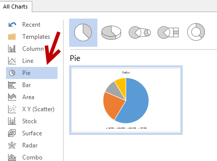
Office: Display Data Labels in a Pie Chart

How to display leader lines in pie chart in Excel? - ExtendOffice 1. Click at the chart, and right click to select Format Data Labels from context menu. 2. In the popping Format Data Labels dialog/pane, check Show Leader Lines in the Label Options section. See screenshot: 3. Close the dialog, now you can see some leader lines appear. If you want to show all leader lines, just drag the labels out of the pie ...

How to Add Data Labels in Excel - Excelchat | Excelchat

Change the format of data labels in a chart To get there, after adding your data labels, select the data label to format, and then click Chart Elements > Data Labels > More Options. To go to the appropriate area, click one of the four icons ( Fill & Line, Effects, Size & Properties ( Layout & Properties in Outlook or Word), or Label Options) shown here.

How to Use Cell Values for Excel Chart Labels

Hide Excel Pivot Table Buttons and Labels 29-01-2020 · Pivot Table With Hidden Buttons and Labels. After those pivot table display options are turned off, here’s what the pivot table looks like. Hide Filters and Show Labels. In the PivotTable Options dialog box, the filter buttons and field labels have to …

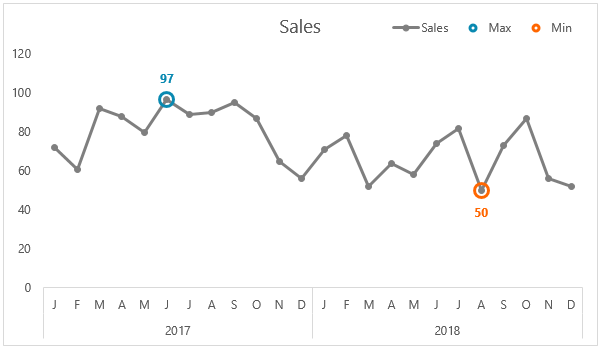
Label Excel Chart Min and Max • My Online Training Hub

Display every "n" th data label in graphs - Microsoft Community With this tool you can assign a range of cells to be the labels for chart series, instead of the Excel defaults. Using a formula, you can have a text show up in every nth cell and then use that range with the XY Chart Labeler to display as the series label. If the full chart labels are in column A, starting in cell A1, then you can use this ...

microsoft excel - Adding data label only to the last value ...

How To Create Labels In Excel - matsubara-seeek.info Make Row Labels In Excel 2007 Freeze For Easier Reading from . Starting document near the bottom. Click a data label one time to select all data labels in a data series or two times to select just one data label that you want to delete, and then press delete. Click finish & merge in the finish group on the mailings tab.

Apply Custom Data Labels to Charted Points - Peltier Tech

Format Data Labels in Excel- Instructions - TeachUcomp, Inc. Then select the "Format Data Labels…" command from the pop-up menu that appears to format data labels in Excel. Using either method then displays the "Format Data Labels" task pane at the right side of the screen. Set the values and positioning of the data labels in the "Label Options" category, which is shown by default.

Display Customized Data Labels on Charts & Graphs

Adding rich data labels to charts in Excel 2013 | Microsoft 365 Blog To add a data label in a shape, select the data point of interest, then right-click it to pull up the context menu. Click Add Data Label, then click Add Data Callout . The result is that your data label will appear in a graphical callout. In this case, the category Thr for the particular data label is automatically added to the callout too.

Format Number Options for Chart Data Labels in PowerPoint ...

How to Add Data Labels to an Excel 2010 Chart - dummies On the Chart Tools Layout tab, click Data Labels→More Data Label Options. The Format Data Labels dialog box appears. You can use the options on the Label Options, Number, Fill, Border Color, Border Styles, Shadow, Glow and Soft Edges, 3-D Format, and Alignment tabs to customize the appearance and position of the data labels.

Directly Labeling in Excel

How to Use Cell Values for Excel Chart Labels - How-To Geek Select the chart, choose the "Chart Elements" option, click the "Data Labels" arrow, and then "More Options." Uncheck the "Value" box and check the "Value From Cells" box. Select cells C2:C6 to use for the data label range and then click the "OK" button. The values from these cells are now used for the chart data labels.

Adding rich data labels to charts in Excel 2013 | Microsoft ...

How to add data labels from different column in an Excel chart? Right click the data series in the chart, and select Add Data Labels > Add Data Labels from the context menu to add data labels. 2. Click any data label to select all data labels, and then click the specified data label to select it only in the chart. 3.

About Data Labels

How to show data label in "percentage" instead of - Microsoft Community Select Format Data Labels Select Number in the left column Select Percentage in the popup options In the Format code field set the number of decimal places required and click Add. (Or if the table data in in percentage format then you can select Link to source.) Click OK Regards, OssieMac Report abuse 8 people found this reply helpful ·

Format Data Labels in Excel- Instructions - TeachUcomp, Inc.

Find, label and highlight a certain data point in Excel scatter graph Here's how: Click on the highlighted data point to select it. Click the Chart Elements button. Select the Data Labels box and choose where to position the label. By default, Excel shows one numeric value for the label, y value in our case. To display both x and y values, right-click the label, click Format Data Labels…, select the X Value and ...