38 pivot table excel row labels side by side
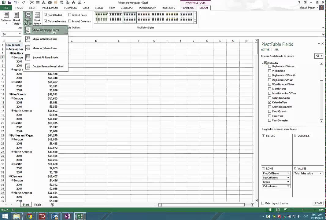
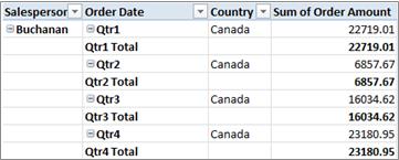
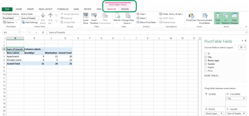
› documents › excelHow to make row labels on same line in pivot table? Click any cell in your pivot table, and the PivotTable Tools tab will be displayed. 2. Under the PivotTable Tools tab, click Design > Report Layout > Show in Tabular Form, see screenshot: 3. And now, the row labels in the pivot table have been placed side by side at once, see screenshot: › publication › ppic-statewide-surveyPPIC Statewide Survey: Californians and Their Government Oct 27, 2022 · Key Findings. California voters have now received their mail ballots, and the November 8 general election has entered its final stage. Amid rising prices and economic uncertainty—as well as deep partisan divisions over social and political issues—Californians are processing a great deal of information to help them choose state constitutional officers and state legislators and to make ...
› data-analysis › chartsHow to Create Charts in Excel (Easy Tutorial) To move the legend to the right side of the chart, execute the following steps. 1. Select the chart. 2. Click the + button on the right side of the chart, click the arrow next to Legend and click Right. Result: Data Labels. You can use data labels to focus your readers' attention on a single data series or data point. 1. Select the chart. 2.

Pivot table excel row labels side by side
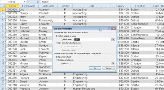
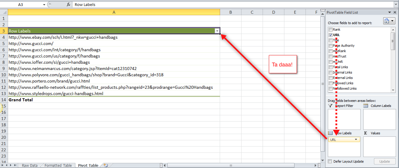
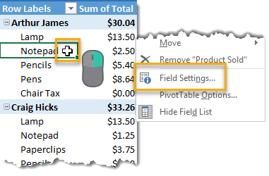
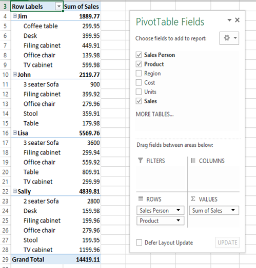
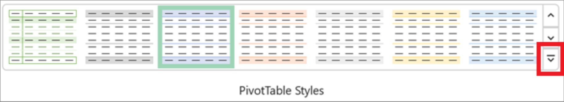
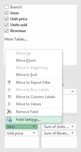
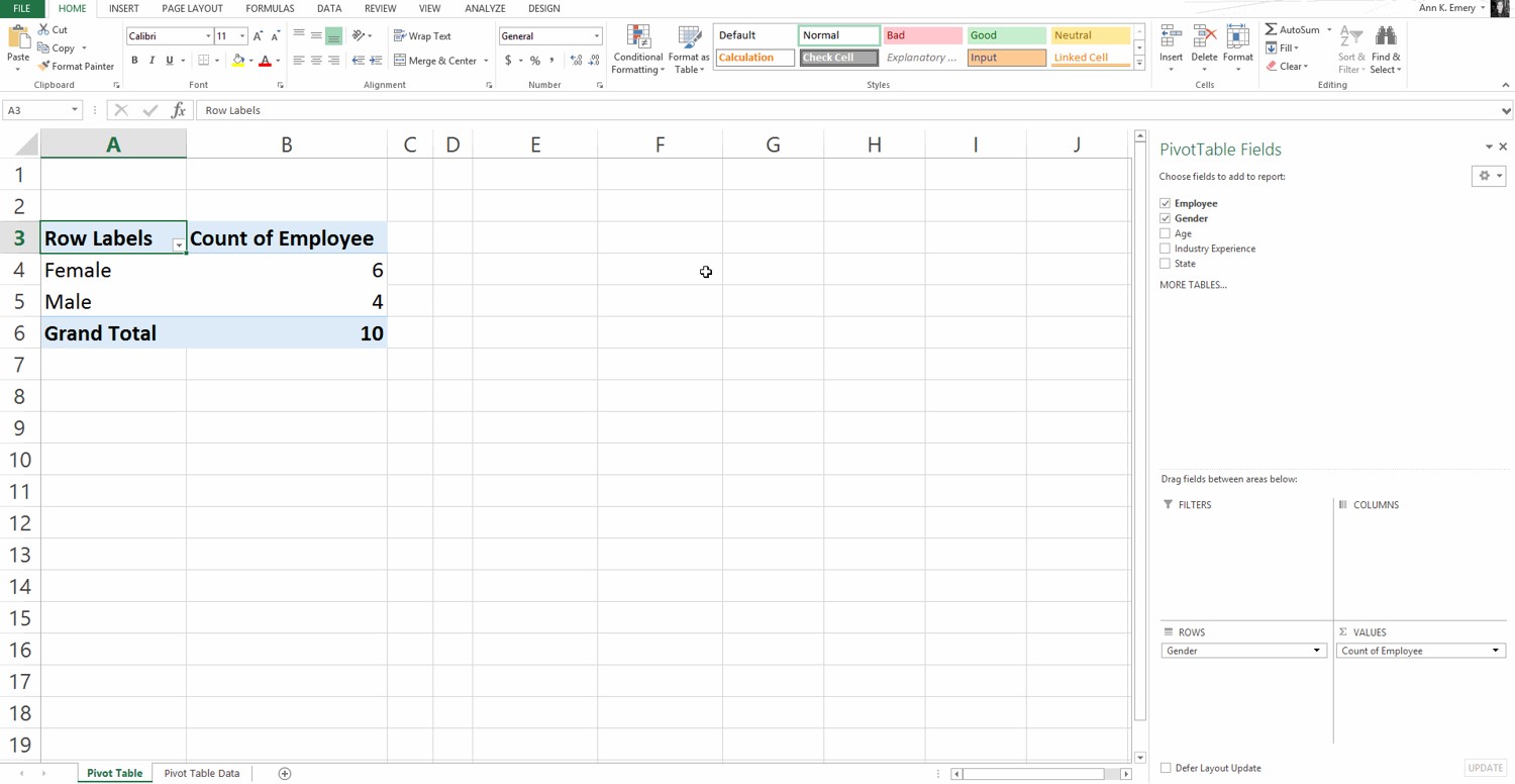
blog.hubspot.com › marketing › how-to-create-pivotHow to Create a Pivot Table in Excel: A Step-by-Step Tutorial Dec 31, 2021 · After you've completed Step 3, Excel will create a blank pivot table for you. Your next step is to drag and drop a field — labeled according to the names of the columns in your spreadsheet — into the Row Labels area. This will determine what unique identifier — blog post title, product name, and so on — the pivot table will organize ... › excel-pivot-tables › how-to-useHow to Use Pivot Table Field Settings and Value Field Setting But that is not all. A dynamic pivot table will reduce work of data maintenance and it will consider all newly added data as the source data. How to Refresh Pivot Charts | To refresh a pivot table we have a simple button of refresh pivot table in the ribbon. Or you can right click on the pivot table. Here's how you do it. Conditional Formatting ... › excel-pivot-table-formatHow to Format Excel Pivot Table - Contextures Excel Tips Jun 22, 2022 · Video: Change Pivot Table Labels. Watch this short video tutorial to see how to make these changes to the pivot table headings and labels. Get the Sample File. No Macros: To experiment with pivot table styles and formatting, download the sample file. The zipped file is in xlsx format, and and does NOT contain any macros.
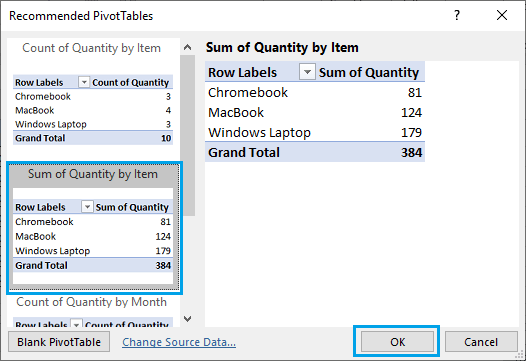
Pivot table excel row labels side by side. › excelpivottablesetupHow to Set Up Excel Pivot Table - Contextures Excel Tips Oct 26, 2022 · This will make it easier for Excel to build the pivot table. Next, click the Insert tab on the Excel Ribbon. There are two pivot table commands in the Tables group, at the left side of the Insert tab: Recommended PivotTables - select a layout and Excel creates a quick pivot table Use this command if you're not too experienced with pivot tables › excel-pivot-table-formatHow to Format Excel Pivot Table - Contextures Excel Tips Jun 22, 2022 · Video: Change Pivot Table Labels. Watch this short video tutorial to see how to make these changes to the pivot table headings and labels. Get the Sample File. No Macros: To experiment with pivot table styles and formatting, download the sample file. The zipped file is in xlsx format, and and does NOT contain any macros. › excel-pivot-tables › how-to-useHow to Use Pivot Table Field Settings and Value Field Setting But that is not all. A dynamic pivot table will reduce work of data maintenance and it will consider all newly added data as the source data. How to Refresh Pivot Charts | To refresh a pivot table we have a simple button of refresh pivot table in the ribbon. Or you can right click on the pivot table. Here's how you do it. Conditional Formatting ... blog.hubspot.com › marketing › how-to-create-pivotHow to Create a Pivot Table in Excel: A Step-by-Step Tutorial Dec 31, 2021 · After you've completed Step 3, Excel will create a blank pivot table for you. Your next step is to drag and drop a field — labeled according to the names of the columns in your spreadsheet — into the Row Labels area. This will determine what unique identifier — blog post title, product name, and so on — the pivot table will organize ...
Excel 2016 Pivot Tables Lab Webinar - ppt download
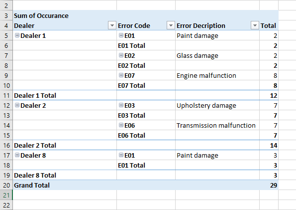
How to Flatten and repeat Row Labels in a Pivot Table
Excel Pivot Table: How To Show Labels Side by Side - YouTube
Design the layout and format of a PivotTable
How to Create a Pivot Table in Excel 2010 - dummies
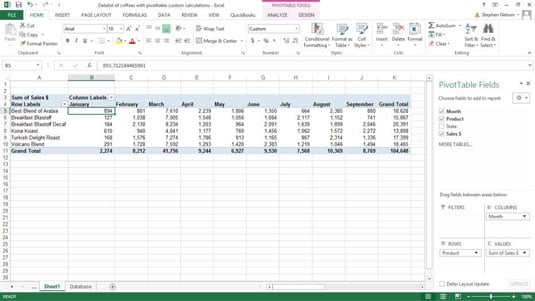
How to Create Custom Calculations for an Excel Pivot Table ...
Design the layout and format of a PivotTable

Analyzing Data in Excel

Creating Pivot Tables in Excel for Exported Data – Teaching ...
Design the layout and format of a PivotTable

Pivot table row labels in separate columns • AuditExcel.co.za
How To Manage Big Data With Pivot Tables
101 Advanced Pivot Table Tips And Tricks You Need To Know ...

Pivot table row labels side by side – Excel Tutorial
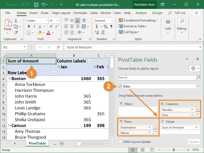
Add Multiple Columns to a Pivot Table | CustomGuide

How can I fill the empty labels with the headings in a Pivot ...

Excel Pivot Table Field Layout Changes Videos Examples
How to Make a Pivot Table in Excel - Excel Master Consultant

Repeat item labels in a PivotTable

Trick to Show Excel Pivot Table Grand Total at Top
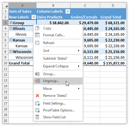
Group Items in a Pivot Table | DevExpress End-User Documentation
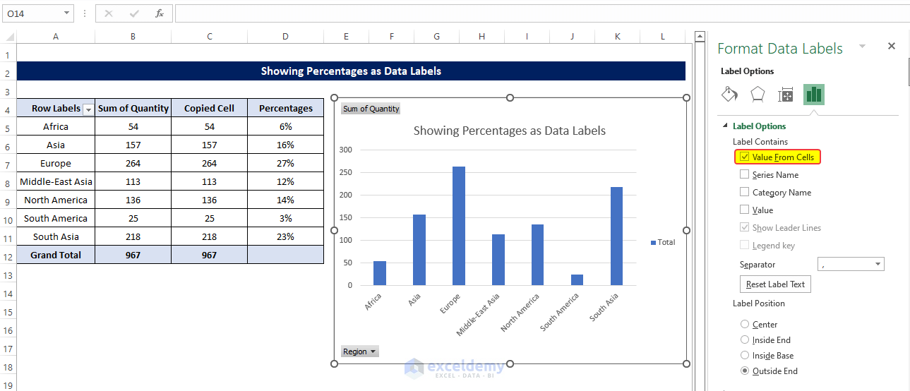
Data Labels in Excel Pivot Chart (Detailed Analysis) - ExcelDemy
Design the layout and format of a PivotTable
How to Create Two Pivot Tables in Single Worksheet

Pivot Tables in Excel
Design the layout and format of a PivotTable
The Pivot table tools ribbon in Excel
How to add side by side rows in excel pivot table ? | AnswerTabs
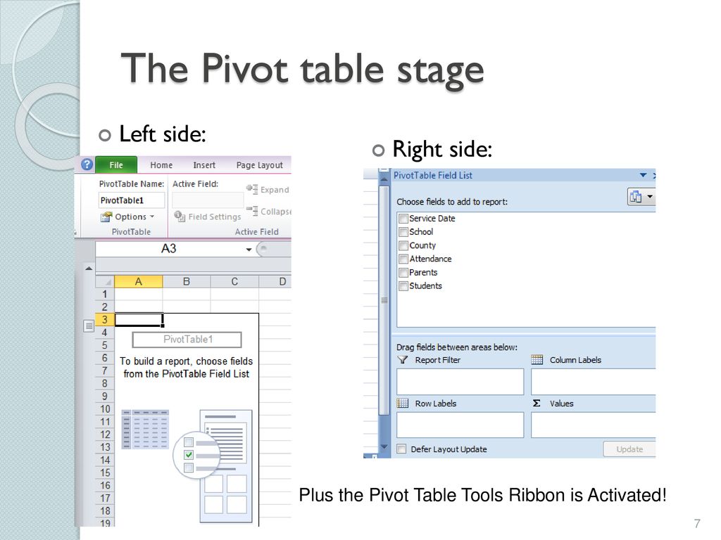
Excel 2016 Pivot Tables Lab Webinar - ppt download

Pivot table row labels in separate columns • AuditExcel.co.za
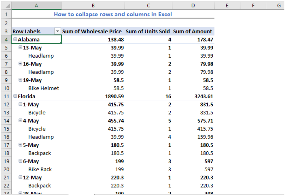
How To Collapse Rows And Columns In Excel - Excelchat | Excelchat

java - Apache POI : Excel Pivot Table - Row Label - Stack ...
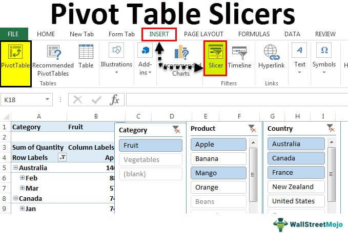
How to Insert Slicer in a Excel Pivot Table? (with Examples)
Pivot table row labels side by side – Excel Tutorial
How to Save Time and Energy by Analyzing Your Data with Pivot ...

Pivot table row labels side by side – Excel Tutorial
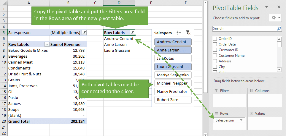
3 Ways to Display (Multiple Items) Filter Criteria in a Pivot ...

Pivot table row labels side by side – Excel Tutorial
Post a Comment for "38 pivot table excel row labels side by side"